

Differential Expression#
This tutorial covers pseudobulk differential expression: summing each sample’s counts across all cells of the same cell type, then testing genes for expression differences between conditions with limma-voom. It uses the same ~10 million cell cytokine stimulation dataset as the other tutorials, comparing IFN-gamma-stimulated cells against phosphate-buffered saline (PBS) controls within each cell type. Download it from the Basic Workflow tutorial — the full object, or a subsampled version to follow along on a laptop.
Note
brisc runs differential expression through limma, an R package that isn’t installed with brisc by default. Install it before running this tutorial — see Installation → R packages.
Loading and quality control#
The experiment spans several cytokines, but this analysis compares only IFN-gamma vs. PBS control, so we pass a custom_filter to qc that keeps just these cells and fails every other cytokine. As in the basic workflow, qc doesn’t drop any cells — it merely records which ones passed in a Boolean passed_QC column.
cast_obs(strict=False) then recasts cytokine as a two-level Enum with PBS first, making PBS the reference that IFN-gamma is compared against. Specifying strict=False ensures that every cytokine not in those two levels becomes null, leaving just PBS and IFN-gamma.
from brisc import SingleCell
import polars as pl

sc = SingleCell(
    'Parse_10M_PBMC_cytokines.h5ad',
    obs_columns=['sample', 'donor', 'cell_type', 'cytokine'])\
    .qc(custom_filter=pl.col('cytokine').is_in(['IFN-gamma', 'PBS']),
        allow_float=True)\
    .cast_obs({'cytokine': pl.Enum(['PBS', 'IFN-gamma'])}, strict=False)
Note
The subsampled dataset already contains only PBS and IFN-gamma cells, so the custom_filter matches every cell and has no effect here. It is kept so the code matches the full-dataset run.
Pseudobulk aggregation#
pseudobulk() sums each gene’s raw counts across all cells from the same sample and cell type. Differential expression (DE) then runs on these per-sample gene expression profiles rather than on individual cells.
Pseudobulk datasets have three slots — X, obs, and var — and each slot is a dictionary where the keys are cell types. For a given cell type, X is a samples × genes matrix of summed counts, obs is a DataFrame of sample-level metadata, and var is a DataFrame of gene-level metadata. obs has a num_cells column indicating how many cells went into each sample’s pseudobulk. Whereas var retains all of the columns from the original SingleCell dataset, obs keeps only the ones that are the same for every cell within a sample, such as donor and cytokine.
pb = sc.pseudobulk('sample', 'cell_type')
print(pb)
Pseudobulk dataset with 18 cell types, each with 22-24 samples (obs) and 40,352 genes (var)
    Cell types: B Intermediate/Memory, B Naive, CD4 Memory, CD4 Naive, CD8
    Memory, CD8 Naive, CD14 Mono, CD16 Mono, HSPC, ILC, MAIT, NK, NK CD56bright,
    NKT, Plasmablast, Treg, cDC, pDC
CD14 monocytes, for instance, have a 24 × 40,352 count matrix and one obs row per sample:
print(pb.obs['CD14 Mono'].head())
shape: (5, 4)
┌──────────────────┬───────────┬────────┬───────────┐
│ sample           ┆ num_cells ┆ donor  ┆ cytokine  │
│ ---              ┆ ---       ┆ ---    ┆ ---       │
│ enum             ┆ u32       ┆ enum   ┆ enum      │
╞══════════════════╪═══════════╪════════╪═══════════╡
│ Donor1_IFN-gamma ┆ 2526      ┆ Donor1 ┆ IFN-gamma │
│ Donor1_PBS       ┆ 16690     ┆ Donor1 ┆ PBS       │
│ Donor2_IFN-gamma ┆ 1285      ┆ Donor2 ┆ IFN-gamma │
│ Donor2_PBS       ┆ 9159      ┆ Donor2 ┆ PBS       │
│ Donor3_IFN-gamma ┆ 965       ┆ Donor3 ┆ IFN-gamma │
└──────────────────┴───────────┴────────┴───────────┘
IFN-gamma samples have far fewer cells than PBS samples; the log2(num_cells) covariate accounts for this in the model.
Saving the pseudobulk
A pseudobulk dataset is a compact summary of the original SingleCell dataset, so saving it is a convenient way to re-run DE later without reloading the raw single-cell data. save() writes each cell type’s X, obs, and var to a directory, and Pseudobulk('directory') reads it back:
# save the full pseudobulk to a directory
pb.save('pseudobulk')

# or save only certain cell types (you can also pass excluded_cell_types=)
pb.save('monocytes', cell_types=['CD14 Mono', 'CD16 Mono'])

# reload without the raw single-cell data
from brisc import Pseudobulk
pb = Pseudobulk('monocytes')
Sample-level quality control#
Pseudobulk datasets also have a qc() method. It runs independently for each cell type, filtering out low-quality samples, genes, and cell types. By default it keeps:
samples with ≥10 cells of that cell type
non-outlier samples where the number of genes with zero counts is less than three standard deviations above the mean
genes detected in ≥80% of samples
cell types with ≥2 samples remaining after applying the above three filters
Passing cytokine as the group column applies the gene-detection filter within each condition, keeping a gene only if it is detected in ≥80% of samples in both IFN-gamma and PBS. Without specifying a group column, that 80% threshold would instead be evaluated across all samples.
pb = pb.qc('cytokine', verbose=True)
[B Intermediate/Memory] Starting with 24 samples and 40,352 genes.
[B Intermediate/Memory] Filtering to samples with at least 10 B Intermediate/Memory cells...
[B Intermediate/Memory] 24 samples remain after filtering to samples with at least 10 B Intermediate/Memory cells.
[B Intermediate/Memory] Filtering to samples where the number of genes with 0 counts is <3 standard deviations above the mean...
[B Intermediate/Memory] 24 samples remain after filtering to samples where the number of genes with 0 counts is <3 standard deviations above the mean.
[B Intermediate/Memory] Filtering to genes with at least one count in 80.0% of samples in each group...
[B Intermediate/Memory] 14,696 genes remain after filtering to genes with at least one count in 80.0% of samples in each group.
...
[Plasmablast] Starting with 22 samples and 40,352 genes.
[Plasmablast] Filtering to samples with at least 10 Plasmablast cells...
[Plasmablast] 11 samples remain after filtering to samples with at least 10 Plasmablast cells.
[Plasmablast] Skipping this cell type because it has only 1 sample where group_column = 'IFN-gamma' after filtering, which is fewer than min_samples (2)
The number of genes kept varies by cell type, and a rare cell type can drop out entirely when a condition is left with too few samples. Here, Plasmablast is skipped because only one IFN-gamma sample has enough cells.
Customizing the filters
Each threshold is configurable:
pb = pb.qc(
    'cytokine', min_cells=20, max_standard_deviations=2,
    min_nonzero_fraction=0.9, min_samples=3)
min_cells, max_standard_deviations, min_nonzero_fraction, and min_samples are the four filters above; pass None to switch a filter off, or min_nonzero_fraction=0 to drop only all-zero genes. Use custom_filter to add an extra per-sample Boolean filter.
Differential expression#
library_size() computes a TMM-normalized library size for each sample, and de() then fits a limma-voom model independently for each cell type. The model is written as an R formula. Each term is the name of a column in obs. brisc passes those columns to R’s model.matrix, which turns the formula into a design matrix.
How a column enters the matrix depends on its type. Numeric columns like log2(num_cells) go in unchanged. Categorical columns — here cytokine and donor — are split into multiple indicator columns, each holding 1 for samples in its category and 0 otherwise. Giving every category its own column is one-hot encoding; R uses the closely related treatment coding, which drops one category, so a column with N categories becomes N − 1 indicators. Each is named by joining the column and category with no separator, so cytokine’s IFN-gamma becomes cytokineIFN-gamma.
The dropped category is the reference, which the model folds into the intercept. For cytokine that’s PBS, the first level of the Enum we built while loading, so the design has a cytokineIFN-gamma column but no cytokinePBS column. This is exactly what we want: the cytokineIFN-gamma coefficient measures IFN-gamma relative to PBS. de reports the first non-intercept coefficient by default, so the call needs nothing but the formula:
pb = pb.library_size()
de = pb.de(
    '~ cytokine + donor + log2(num_cells) + log2(library_size)',
    verbose=True)
[B Intermediate/Memory] Validating formula...
[B Intermediate/Memory] Creating design matrix...
[B Intermediate/Memory] Validating coefficient...
[B Intermediate/Memory] Defining groups...
[B Intermediate/Memory] Grouping on the 'cytokine' column of obs.
[B Intermediate/Memory] Converting the expression matrix, library sizes and groups to R...
[B Intermediate/Memory] Running voomByGroup...
[B Intermediate/Memory] Running lmFit...
[B Intermediate/Memory] Running eBayes...
[B Intermediate/Memory] Collating results...

[B Naive] Validating formula...
[B Naive] Creating design matrix...
[B Naive] Validating coefficient...
[B Naive] Defining groups...
[B Naive] Grouping on the 'cytokine' column of obs.
[B Naive] Converting the expression matrix, library sizes and groups to R...
[B Naive] Running voomByGroup...
[B Naive] Running lmFit...
[B Naive] Running eBayes...
[B Naive] Collating results...
...
In the formula, cytokine is the effect of interest, donor accounts for the fact that there are multiple donor individuals, and log2(num_cells) and log2(library_size) — recommended for every pseudobulk model — correct for the number of cells aggregated and for sequencing depth. Because the effect of interest is categorical, de fits voom’s mean-variance trend separately within each condition (a method called voomByGroup) by default.
de tests only the cell types that survived QC, so Plasmablast (dropped above) isn’t among them. By default it also silently skips any surviving cell type where the differential expression model would fail to converge, e.g. due to having more covariates than samples; pass strict=True to raise an error instead, or drop such cell types yourself with drop_cell_types().
How R codes categorical and ordinal columns
By default, R applies the treatment coding above (contr.treatment) to String, Categorical, and Enum columns, and leaves numeric columns as-is. Two arguments change how a specific column is coded:
ordinal_columns— specifies columns whose levels have an order, like dose, timepoint, or severity. Instead of an indicator per category, R fits a trend across the levels (contr.poly): a linear term (column_name.L), a quadratic term (column_name.Q), and so on, assuming the levels are evenly spaced. For example, a steady dose response shows up incolumn_name.L.categorical_columns— specifies integer columns to treat as categorical (treatment-coded) instead of numeric.
To change the coding globally instead, set R’s contrasts option before calling de — to any of R’s contrast-coding schemes (Helmert, sum-to-zero, and so on):
from ryp import r
r('options(contrasts = c(unordered = "contr.treatment", '
  'ordered = "contr.helmert"))')
Other DE options
group=Falseuses a single mean-variance trend (plain voom) rather than voomByGroup.robust=Truemakes the empirical Bayes step robust to outlier samples.strict=Trueerrors on any cell type whose design matrix is rank-deficient or has too few samples to fit its coefficients — by default these cell types are silently skipped.return_voom_info=Falseskips storing the voom weights and plot data, for lower memory and runtime when you don’t need them.cell_typesandexcluded_cell_typesrestrict testing to a subset of cell types.categorical_columnsandordinal_columnschange how specific columns are coded in the design matrix (see the box above).formula,coefficient,contrasts, andgroupcan be dictionaries keyed by cell type, to allow different cell types to have different designs (e.g. when a covariate is present in only some cell types).
Exploring the results#
The results are collected in a DE object. get_num_hits() counts the significant genes (FDR < 0.05) in each cell type; cell types with no hits are omitted.
print(de.get_num_hits())
shape: (4, 2)
┌───────────────────────┬──────────┐
│ cell_type             ┆ num_hits │
│ ---                   ┆ ---      │
│ str                   ┆ u32      │
╞═══════════════════════╪══════════╡
│ B Intermediate/Memory ┆ 1        │
│ B Naive               ┆ 375      │
│ CD14 Mono             ┆ 661      │
│ CD16 Mono             ┆ 403      │
└───────────────────────┴──────────┘
B cells and monocytes respond most strongly, as expected for IFN-gamma; the other tested cell types show no hits at this significance threshold.
get_hits() returns the hits themselves; the num_top_hits parameter caps how many it reports per cell type. Each row is one gene in one cell type: logFC is the log2 fold change (the effect size), SE its standard error, LCI/UCI its 95% confidence interval, and AveExpr the gene’s average expression in log CPM; p, Bonferroni, and FDR are the raw and corrected p-values, and coefficient names the tested effect.
print(de.get_hits(num_top_hits=5))
shape: (16, 11)
┌───────────────────────┬───────────────────┬─────────┬───────────┬──────────┬────────────┬───────────┬──────────┬──────────┬────────────┬──────────┐
│ cell_type             ┆ coefficient       ┆ gene    ┆ logFC     ┆ SE       ┆ LCI        ┆ UCI       ┆ AveExpr  ┆ p        ┆ Bonferroni ┆ FDR      │
│ ---                   ┆ ---               ┆ ---     ┆ ---       ┆ ---      ┆ ---        ┆ ---       ┆ ---      ┆ ---      ┆ ---        ┆ ---      │
│ str                   ┆ str               ┆ str     ┆ f64       ┆ f64      ┆ f64        ┆ f64       ┆ f64      ┆ f64      ┆ f64        ┆ f64      │
╞═══════════════════════╪═══════════════════╪═════════╪═══════════╪══════════╪════════════╪═══════════╪══════════╪══════════╪════════════╪══════════╡
│ B Intermediate/Memory ┆ cytokineIFN-gamma ┆ TENM4   ┆ -6.541458 ┆ 0.904791 ┆ -8.461154  ┆ -4.621763 ┆ 5.045181 ┆ 0.000002 ┆ 0.031375   ┆ 0.031375 │
│ B Naive               ┆ cytokineIFN-gamma ┆ LAP3    ┆ 7.407211  ┆ 1.320611 ┆ 4.602272   ┆ 10.21215  ┆ 7.001164 ┆ 0.000043 ┆ 0.648348   ┆ 0.007978 │
│ B Naive               ┆ cytokineIFN-gamma ┆ CASP10  ┆ 5.91294   ┆ 1.294467 ┆ 3.16353    ┆ 8.66235   ┆ 6.22115  ┆ 0.000334 ┆ 1.0        ┆ 0.025158 │
│ B Naive               ┆ cytokineIFN-gamma ┆ CFLAR   ┆ 3.227118  ┆ 0.691294 ┆ 1.758831   ┆ 4.695406  ┆ 8.286078 ┆ 0.000273 ┆ 1.0        ┆ 0.023158 │
│ B Naive               ┆ cytokineIFN-gamma ┆ NFIX    ┆ 4.034166  ┆ 0.997575 ┆ 1.915345   ┆ 6.152986  ┆ 3.726182 ┆ 0.000982 ┆ 1.0        ┆ 0.044351 │
│ B Naive               ┆ cytokineIFN-gamma ┆ REV3L   ┆ -2.426383 ┆ 0.602491 ┆ -3.706056  ┆ -1.146709 ┆ 7.312945 ┆ 0.001017 ┆ 1.0        ┆ 0.044849 │
│ CD14 Mono             ┆ cytokineIFN-gamma ┆ CFH     ┆ 8.416471  ┆ 1.822179 ┆ 4.460555   ┆ 12.372386 ┆ 3.082946 ┆ 0.000543 ┆ 1.0        ┆ 0.035723 │
│ CD14 Mono             ┆ cytokineIFN-gamma ┆ LAP3    ┆ 5.340516  ┆ 0.965731 ┆ 3.243932   ┆ 7.437099  ┆ 9.694517 ┆ 0.000115 ┆ 1.0        ┆ 0.026415 │
│ CD14 Mono             ┆ cytokineIFN-gamma ┆ CASP10  ┆ 3.927575  ┆ 0.699754 ┆ 2.408423   ┆ 5.446727  ┆ 6.461136 ┆ 0.000101 ┆ 1.0        ┆ 0.026415 │
│ CD14 Mono             ┆ cytokineIFN-gamma ┆ CD38    ┆ 9.551953  ┆ 1.913129 ┆ 5.398585   ┆ 13.705321 ┆ 8.810696 ┆ 0.000283 ┆ 1.0        ┆ 0.031859 │
│ CD14 Mono             ┆ cytokineIFN-gamma ┆ PDK4    ┆ -9.347026 ┆ 2.237785 ┆ -14.205216 ┆ -4.488837 ┆ 2.094128 ┆ 0.001197 ┆ 1.0        ┆ 0.04558  │
│ CD16 Mono             ┆ cytokineIFN-gamma ┆ LAP3    ┆ 2.727379  ┆ 0.446265 ┆ 1.776283   ┆ 3.678475  ┆ 9.924472 ┆ 0.00002  ┆ 0.277314   ┆ 0.010575 │
│ CD16 Mono             ┆ cytokineIFN-gamma ┆ CD38    ┆ 5.540838  ┆ 1.031595 ┆ 3.342265   ┆ 7.739412  ┆ 9.321841 ┆ 0.000078 ┆ 1.0        ┆ 0.014432 │
│ CD16 Mono             ┆ cytokineIFN-gamma ┆ ST3GAL1 ┆ -1.436892 ┆ 0.364966 ┆ -2.214721  ┆ -0.659064 ┆ 8.076972 ┆ 0.001315 ┆ 1.0        ┆ 0.047342 │
│ CD16 Mono             ┆ cytokineIFN-gamma ┆ ETV7    ┆ 4.134528  ┆ 0.825406 ┆ 2.375394   ┆ 5.893663  ┆ 5.994346 ┆ 0.000155 ┆ 1.0        ┆ 0.019453 │
│ CD16 Mono             ┆ cytokineIFN-gamma ┆ PLAUR   ┆ -1.609256 ┆ 0.340264 ┆ -2.334438  ┆ -0.884073 ┆ 6.608727 ┆ 0.000268 ┆ 1.0        ┆ 0.024208 │
└───────────────────────┴───────────────────┴─────────┴───────────┴──────────┴────────────┴───────────┴──────────┴──────────┴────────────┴──────────┘
Classic interferon-stimulated genes recur across cell types: LAP3 is a top hit in three of the four, and CD38 in both monocyte subsets — both are canonical interferon targets induced by IFN-gamma.
plot_volcano() plots fold change against significance for one cell type. CD14 monocytes mount one of the strongest responses to IFN-gamma:
de.plot_volcano('CD14 Mono', 'volcano.png')
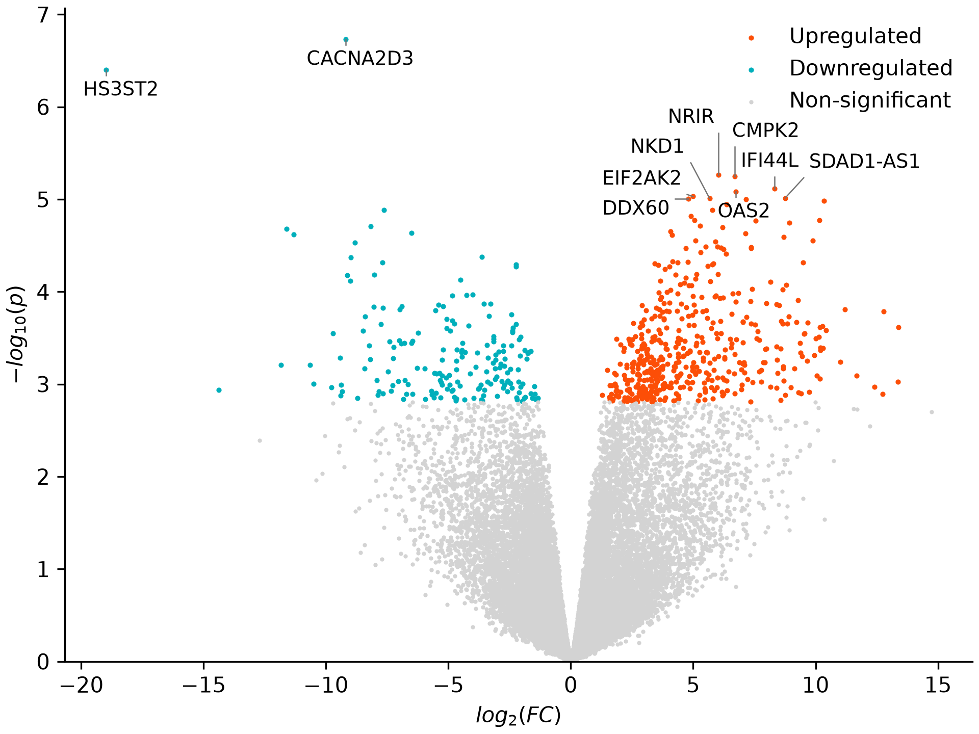
de.table is the complete result as a polars DataFrame — every tested gene in every cell type, not only the hits. Sort, filter, and select it like any polars DataFrame; here, sorted by FDR:
print(de.table.sort('FDR').head())
shape: (5, 11)
┌───────────┬───────────────────┬─────────────────┬───────────┬──────────┬───────────┬───────────┬──────────┬───────────┬────────────┬──────────┐
│ cell_type ┆ coefficient       ┆ gene            ┆ logFC     ┆ SE       ┆ LCI       ┆ UCI       ┆ AveExpr  ┆ p         ┆ Bonferroni ┆ FDR      │
│ ---       ┆ ---               ┆ ---             ┆ ---       ┆ ---      ┆ ---       ┆ ---       ┆ ---      ┆ ---       ┆ ---        ┆ ---      │
│ str       ┆ str               ┆ str             ┆ f64       ┆ f64      ┆ f64       ┆ f64       ┆ f64      ┆ f64       ┆ f64        ┆ f64      │
╞═══════════╪═══════════════════╪═════════════════╪═══════════╪══════════╪═══════════╪═══════════╪══════════╪═══════════╪════════════╪══════════╡
│ B Naive   ┆ cytokineIFN-gamma ┆ CYP2J2          ┆ 13.502077 ┆ 1.424344 ┆ 10.476812 ┆ 16.527342 ┆ 2.316806 ┆ 7.0399e-8 ┆ 0.001068   ┆ 0.001068 │
│ B Naive   ┆ cytokineIFN-gamma ┆ OASL            ┆ 10.644854 ┆ 1.280494 ┆ 7.925123  ┆ 13.364585 ┆ 5.743191 ┆ 3.9755e-7 ┆ 0.006032   ┆ 0.002011 │
│ B Naive   ┆ cytokineIFN-gamma ┆ ENSG00000271955 ┆ 9.816521  ┆ 1.174002 ┆ 7.322975  ┆ 12.310066 ┆ 4.601677 ┆ 3.6876e-7 ┆ 0.005596   ┆ 0.002011 │
│ B Naive   ┆ cytokineIFN-gamma ┆ LY6E-DT         ┆ 8.979601  ┆ 1.125847 ┆ 6.588335  ┆ 11.370868 ┆ 5.250673 ┆ 6.7586e-7 ┆ 0.010255   ┆ 0.002564 │
│ B Naive   ┆ cytokineIFN-gamma ┆ TBX21           ┆ 9.276725  ┆ 1.319861 ┆ 6.473378  ┆ 12.080072 ┆ 3.216798 ┆ 0.000003  ┆ 0.049237   ┆ 0.003363 │
└───────────┴───────────────────┴─────────────────┴───────────┴──────────┴───────────┴───────────┴──────────┴───────────┴────────────┴──────────┘
Saving the results
A DE object can be written to a directory and read back later, so you don’t have to re-run the model to revisit the results. save() writes the table and any voom info, and DE('directory') reads it back:
Other result options
plot_voom()draws the mean-variance trend that voom fits, with one curve per group when using voomByGroup.significance_column='Bonferroni'or a lowerthresholdinget_hitsandplot_volcanogives a stricter set of DE genes.
Differential expression with complex designs#
The default coefficient reports one comparison — a single condition against the baseline. A contrast tests any linear combination of the design-matrix columns instead: an average of several conditions, the difference between two of them, or a whole panel of comparisons at once. You write each as an expression in the contrasts argument, and de evaluates it.
The interferons are a good example. The dataset has 90 cytokines, and the four type I interferons — IFN-alpha1, IFN-beta, IFN-epsilon, IFN-omega — all signal through the IFNAR receptor, while IFN-gamma (type II) signals through IFNGR. How do their responses differ? That asks for the average of the four type I coefficients minus the IFN-gamma coefficient — a combination no single coefficient can give, and just what contrasts is for.
For those coefficients to exist, drop the intercept with ~ 0 + cytokine so every interferon gets its own column. With an intercept, treatment coding leaves one level out as the reference, so it gets no column — and a contrast that names it would fail with “not the name of a column of the design matrix”. Then, specify the contrast using the contrasts argument. contrasts asks for a dictionary where the keys are the names of the contrasts (name them whatever you’d like; this only affects the name of the coefficient in the final DE object) and the values are strings containing mathematical formulas that reference columns of the design matrix. Note that unlike in R formulas, backticks are never required, even when referencing columns that would not be valid R variable names.
from brisc import SingleCell
import polars as pl

interferons = ['IFN-alpha1', 'IFN-beta', 'IFN-epsilon', 'IFN-omega', 'IFN-gamma']

sc = SingleCell(
    'Parse_10M_PBMC_cytokines.h5ad',
    obs_columns=['sample', 'donor', 'cell_type', 'cytokine'])\
    .qc(custom_filter=pl.col('cytokine').is_in(interferons),
        allow_float=True)

pb = sc.pseudobulk('sample', 'cell_type')\
    .qc('cytokine')\
    .library_size()

de = pb.de(
    '~ 0 + cytokine + donor + log2(num_cells) + log2(library_size)',
    contrasts={'Type I vs II':
        '(cytokineIFN-alpha1 + cytokineIFN-beta'
        ' + cytokineIFN-epsilon + cytokineIFN-omega)/4'
        ' - cytokineIFN-gamma'})
The same approach can be used to express any linear combination of coefficients — one cytokine family against another, or several comparisons at once by adding more entries to the dictionary.
Pipeline summary#
The full differential expression pipeline:
from brisc import SingleCell
import polars as pl

sc = SingleCell(
    'Parse_10M_PBMC_cytokines.h5ad', num_threads=-1,
    obs_columns=['sample', 'donor', 'cell_type', 'cytokine'])\
    .qc(custom_filter=pl.col('cytokine').is_in(['IFN-gamma', 'PBS']),
        allow_float=True)\
    .cast_obs({'cytokine': pl.Enum(['PBS', 'IFN-gamma'])}, strict=False)

pb = sc.pseudobulk('sample', 'cell_type')\
    .qc('cytokine')\
    .library_size()

de = pb.de('~ cytokine + donor + log2(num_cells) + log2(library_size)')

de.plot_volcano('CD14 Mono', 'volcano.png')
Step |
Method |
What it does |
|---|---|---|
Load |
|
Read data from any supported format |
Quality control |
Filter low-quality cells |
|
Pseudobulk |
Sum raw counts per sample × cell type |
|
Sample QC |
Filter low-quality samples and genes per group |
|
Library size |
Compute TMM-normalized library sizes |
|
Differential expression |
Fit a limma-voom model per cell type |
|
Volcano plot |
Plot fold change against significance for one cell type |